An origin of the laminated structure of ozone
in the lower stratosphere
Y. Tomikawa
Department of Earth and Planetary Science, Graduate School of Science, University of Tokyo, Tokyo 113-0033, Japan
K. Sato
National Institute of Polar Research, Tokyo 173-8515, Japan
M. Fujiwara
Graduate School of Environmental Earth Science, Hokkaido University, Sapporo 060-0810, Japan
K. Kita
Research Center for Advanced Science and Technology, University of Tokyo, Tokyo 153-0041, Japan
M. Yamamori
Center for Climate System Research, University of Tokyo, Tokyo 153-8904, Japan
M. Yoshiki
Department of Geophysics, Kyoto University, Kyoto 606-8502, Japan
Abstract.
Ozonesonde observations at a time interval of 8 hours were conducted at Shigaraki (34.9°N, 136.1°E), Japan during 16-24 April 1998 to investigate the temporal variability of ozone in the midlatitude lower stratosphere. During the observation period, an ozone lamina with a thickness of 2-3 km appeared and ascended with a speed of about 1 km day-1 in the height region of 18-21 km. A trajectory analysis and reverse domain filling calculations indicate that this ozone lamina was caused by the differential advection due to the vertical shear of the subtropical westerly-jet and the embedded stationary Rossby wave therein.
1. Introduction
Laminated structures have often been seen in the vertical profiles of ozone obtained by ozonesonde observations. Previous statistical studies showed that such ozone laminae are most commonly observed from winter to spring in the lower stratosphere at middle and high latitudes [Dobson, 1973; Reid and Vaughan, 1991, 1993]. However, the process to cause this structure has not been established because their temporal evolution is not known in detail. Thus, we conducted an intensive and continuous ozonesonde observation at Shigaraki (34.9°N, 136.1°E), Japan in April 1998, and succeeded in detecting an ascending ozone lamina in the lower stratosphere. In this paper, we show several characteristics of the ozone lamina and examine possible causes of the formation of the ozone lamina.
2. Variations of Ozone Mixing Ratio
An intensive and continuous observation with ozonesondes, radiosondes and the MU (Middle and Upper atmosphere) radar was conducted at Shigaraki (34.9°N, 136.1°E), Japan from 16 to 24 April 1998. Vaisala RS-80 meteorological radiosondes were used to measure the vertical profiles of atmospheric pressure, temperature and humidity. The vertical distributions of atmospheric ozone concentration were obtained with EN-SCI balloonborne electrochemical concentration cell (ECC) ozonesondes connected with the Vaisala RS-80 radiosondes [Komhyr et al., 1995]. The data sampling time is about 1 second with an ascending speed of about 5 m s-1. In this paper, we used data interpolated with a constant vertical interval of 50 m. We launched 24 ozonesondes every 8 hours during the observation period, and most of them reached altitudes over 30 km. The continuous wind measurement was made with the MU radar in the height region of 1-24 km during the observation period. Zonal, meridional and vertical winds were estimated every 30 min. Details of the MU radar system are described by Fukao et al. [1985].
Figure 1 presents the time-height section of ozone mixing ratio obtained by ozonesonde observations at Shigaraki. Potential temperature (θ) is used as a vertical coordinate. Approximate altitudes are also shown. An ozone-enhanced layer with a thickness of 40-60 K in θ (2-3 km in height) appeared at θ = 430 K (17-18 km) on 18 April, and the layer ascended until 21 April (about 25 K day-1 ≈ 1 km day-1). An ozone-depleted layer was seen above the ozone-enhanced layer and disappeared on 19 April. The ozone mixing ratio at 460 K varied from 0.9 ppmv (= parts per million by volume) to 2.1 ppmv during the observation period.
3. Backward Trajectory Analysis
The ozone depletion has often been observed within the Arctic polar vortex in the last decade. It leads to the decrease of ozone mixing ratio with latitude in the lower stratosphere. To see the effect of Arctic ozone depletion in the spring of 1998, Figure 2 shows polar plots of potential vorticity (hereafter referred to as PV) on the 460 K isentropic surface based on operational data by the European Center for Medium-range Weather Forecasts (ECMWF) and the total ozone on 17 April 1998. There is no sharp PV gradient as characterizes the winter polar vortex edge in Fig. 2a. The ozone depletion was mostly recovered by mid-April (Fig. 2b). Therefore, it is considered that the ozone mixing ratio increased with latitude and altitude in the lower stratosphere during the observation period.
Because the variability of large-scale vertical motions in the stratosphere is expected to be too small to make the observed irregularity in ozone mixing ratio, we can deduce that the ozone rich and poor air parcels would be quasi-horizontally advected from high and low latitudes, respectively. In order to examine the origins of the air parcels observed over Shigaraki, we made a backward trajectory analysis using a numerical code developed at National Space Development Agency of Japan (NASDA)/ Earth Observation Research Center (EORC). The calculation is based on temperature and winds of the ECMWF operational analysis on 10 isobaric levels between 400 hPa and 10 hPa. Data are given every 12 hours on a 2.5°× 2.5° horizontal mesh and interpolated linearly in space and time as other trajectory codes [e.g., Knudsen et al., 1996]. A second-order Runge-Kutta scheme with a time step of 1 hour is employed for trajectory integration. The backward trajectories are computed on 10 isentropic surfaces from 400 K to 580 K with a 20 K spacing in potential temperature. Because the reliable period of isentropic trajectory is at most 10 days in the lower stratosphere [cf., Knudsen et al., 1994] and the lifetime of ozone lamina is a few weeks [Reid et al., 1998], the period of trajectory calculation is set to 10 days.
Figure 3 shows the backward trajectories from Shigaraki started at 19Z on 19 April when the ozone mixing ratio was enhanced between 450 K and 490 K (around 18.5-20 km). The trajectories at 460 K and 480 K show that the air parcels with high ozone mixing ratio came from high latitudes (north of 50°N), while the trajectories at 420 K, 440 K, 500 K and 520 K show that the air parcels with low ozone mixing ratio came from low latitudes. This result suggests that the observed ozone variation was caused by the advection from different latitude regions. However, because each trajectory often exhibits a large dispersion [e.g., Newman et al., 1996], another method needs to be used to confirm the result of trajectory analysis.
4. Reverse Domain Filling
PV is commonly used to examine stratospheric processes because it is quasi-conserved for following motions over a few weeks [Andrews et al., 1987]. It is difficult to interpret vertical distributions of PV because of its exponential growth with height in the stratosphere. This difficulty can be overcome using an alternative form of PV which has the properties of conventional PV, but does not increase in magnitude with height as rapidly as PV. Hereafter, this alternative form of PV will be referred to as modified potential vorticity (MPV = PV×θ/θ0-9/2 where θ0 is set to 420 K [Lait, 1994]). As both the ozone mixing ratio and MPV usually increase with latitude in the lower stratosphere, the both quantities would have a positive correlation for meridional motions there. Figure 4 shows the time-height section of MPV at the nearest grid point (35°N, 135°E) from Shigaraki computed with the ECMWF data. The large values of MPV can be seen in the lower part of Fig. 4. However, it is not corresponding to the ozone lamina but to the cut-off cyclone in the troposphere (not shown), because the largest values of MPV is located below the 400 K isentropic surface and its ascent rate is clearly different from that of the ozone lamina (see Fig. 1). In the height region where the ozone lamina was observed, available isobaric levels for calculation are only 3 levels (100 hPa, 70 hPa and 50 hPa), corresponding to the vertical resolution of about 6 km. Because the thickness of the ozone lamina is 2-3 km, the vertical resolution of ECMWF data is too coarse to describe the laminated structure in MPV.
Combining both MPV and backward trajectories, it is possible to show "high-resolution" vertical cross sections of the flow field. Hereafter, this technique is referred to as reverse domain filling (RDF). In RDF, the parcels on 10 isentropic levels (400-580 K) are advected backward from Shigaraki over 7 days. The analyzed MPV data on 7 days earlier date are then interpolated to the end points of the trajectories. These interpolated MPV values are plotted onto the initial points of backward trajectories. According to theoretical experiments, the typical e-folding time for vertical scale reduction is about 4 days in the lower stratosphere [Haynes and Anglade, 1997; Thuburn and Tan, 1997] and the vertical resolution of MPV field calculated with the ECMWF data is about 6 km, implying that RDF calculations may produce the MPV field with the vertical resolution of about 1 km. Figure 5 shows the time-height section of MPV over Shigaraki reconstructed by RDF. Displayed patterns in Fig. 1 and Fig. 5 are similar. High and low MPV values in Fig. 5 correspond to high and low ozone mixing ratios in Fig. 1, respectively. The region of high MPV values moves upward in the same way as the ozone-enhanced layer. The result indicates that the ozone lamina was caused by differential advection interleaving vertically air parcels from different latitude regions.
5. Characteristics of Large-scale Flow and Differential Advection
To examine what flow caused the differential advection, we show the Montgomery potential on the 420 K, 460 K and 500 K isentropic surfaces at 0Z on 16 April 1998 in Fig. 6. The Montgomery potential is defined by:
M = cpT+φ
where cp is the specific heat at constant pressure, T temperature and φ geopotential. On an isentropic surface, the Montgomery potential is the stream function of the geostrophic wind, which then blows along its contours. A similar large-scale wavy structure can be seen in the longitude region of 70°E-160°E (about 8,000 km) in each figures, although the wind speeds along contours are smaller with altitude because of the vertical shear of the subtropical westerly-jet in the lower stratosphere. Its vertical coherence and horizontal scale indicate that this wavy structure is due to a barotropic Rossby wave. Large-scale air parcel motions are determined by the cumulative effects of advection instead of instantaneous one. However, since this structure was nearly stationary and maintained during 13-18 April (not shown), the result of backward trajectory analysis can be interpreted using these instantaneous flow fields. Comparing those contours in Fig. 6 with the backward trajectories in Fig. 3, some features of each trajectory can be explained as follows:
- On the 420 K and 440 K isentropic surfaces, air parcels were advected from 30°E to 110°E owing to the strong westerly-jet while the stationary Rossby wave was existing, and made the wave-like trajectory patterns in the latitude region of 30°N-50°N.
- Air parcels at 460 K and 480 K were located around 60°E on 13 April, and advected to 120°E by 18 April. Since, in this longitude region, the southward wind of the Rossby wave was dominated (see Fig. 6b), the air parcels on these 2 levels were advected from 55°N to 30°N.
- At 500 K and 520 K, air parcels were affected only by the weak northward wind between 90°E and 135°E (see Fig. 6c), and advected from 20°N to Shigaraki.
Thus, the differential advection was caused by the vertical shear of the subtropical westerly-jet and the embedded stationary Rossby wave. This scenario explains well that ozone enhancement was seen only in the height region around 460 K.
6. Summary and Concluding Remarks
The previous studies of ozone laminae were based on the instantaneous vertical profiles of ozone mixing ratio. Thus, to investigate the temporal variability of vertical ozone profiles in the midlatitude lower stratosphere, we have performed an intensive and continuous observation with ozonesondes at Shigaraki, Japan in April 1998. During the observation period, we detected an ozone lamina with a thickness of 2-3 km ascending with a speed of about 1 km day-1 in the height region of 18-21 km.
The contribution of large-scale quasi-isentropic motions was examined. A trajectory analysis and RDF calculations showed that the ozone lamina was formed by the differential advection due to the vertical shear of the subtropical westerly-jet and the embedded stationary Rossby wave.
Whether the fragments of high and low MPV air are finally mixed into ambient air or not is an important issue. A wave breaking causes a rapid and irreversible deformation of material contours [cf., McIntyre and Palmer, 1984}], leading to the substantial mixing with ambient air. On the other hand, if material contours are only perturbed by Rossby or gravity waves, mixing will not occur. This means that the existence of laminae does not necessarily represent an occurrence of mixing. This fact makes it difficult to study ozone laminae, and further researches will be needed.
Acknowledgments
Some ozonesondes launched at Shigaraki were financially supported by T. Sano at NASDA/EORC. The observation was performed by N. Takegawa and S. Matsukawa together with authors. We thank H. Hashiguchi and S. Ogino for their help during observation. We also acknowledge N. Iwagami for his helpful comments and encouragement, and S. Kawakami for his guidance of trajectory analysis. The MU radar belongs to and is operated by Radio Science Center for Space and Atmosphere of Kyoto University. GFD-DENNOU Library was used for drawing figures.
References
Andrews, D. G., J. R. Holton, and C. B. Leovy, Middle Atmosphere Dynamics, 489 pp., Academic, San Diego, Calif., 1987.
Dobson, G. M. B., The laminated structure of the ozone in the atmosphere, Q. J. Roy. Meteorol. Soc., 99, 599-607, 1973.
Fukao, S., T. Sato, T. Tsuda, S. Kato, K. Wakasugi, and T. Makihira, The MU radar with an active phased array system, 1. Antenna and power amplifiers, Radio Sci., 20, 1155-1168, 1985.
Haynes, P., and J. Anglade, The Vertical-Scale Cascade in Atmospheric Tracers due to Large-Scale Differential Advection, J. Atmos. Sci., 54, 1121-1136, 1997.
Knudsen, B. M., and G. D. Carver, Accuracy of the isentropic trajectories calculated for the EASOE campaign, Geophys. Res. Lett., 21, 1199-1202, 1994.
Knudsen, B. M., J. M. Rosen, N. T. Kjome, and A. T. Whitten, Comparison of analyzed stratospheric temperatures and calculated trajectories with long-duration balloon data, J. Geophys. Res., 101, 19137-19145, 1996.
Komhyr, W. D., R. A. Barnes, G. B. Brothers, J. A. Lathrop, and D. P. Opperman, Electrochemical concentration cell ozonesonde performance evaluation during STOIC 1989, J. Geophys. Res., 100, 9231-9244, 1995.
Lait, L. R., An Alternative Form for Potential Vorticity, J. Atmos. Sci., 51, 1754-1759, 1994.
McIntyre, M. E., and T. N. Palmer, The 'surf zone' in the stratosphere, J. Atmos. Terr. Phys., 46, 825-849, 1984.
Newman, P. A., L. R. Lait, M. R. Schoeberl, M. Seablom, L. Coy, R. Rood, R. Swinbank, M. Proffitt, M. Loewenstein, J. R. Podolske, J. W. Elkins, C. R. Webster, R. D. May, D. W. Fahey, G. S. Dutton, and K. R. Chan, Measurements of polar vortex air in the midlatitudes, J. Geophys. Res., 101, 12879-12891, 1996.
Reid, S. J., and G. Vaughan, Lamination in ozone profiles in the lower stratosphere, Q. J. Roy. Meteorol. Soc., 117, 825-844, 1991.
Reid, S. J., and G. Vaughan, Occurrence of Ozone Laminae Near the Boundary of the Stratosphere Polar Vortex, J. Geophys. Res., 98, 8883-8890, 1993.
Reid, S. J., M. Rex, P. Von der Gathen, I. Fløisand, F. Stordal, G. D. Carver, A. Beck, E. Reimer, R. Krüger-Carstensen, L. L. de Haan, G. Braathen, V. Dorokhov, H. Fast, E. Kyrö, M. Gil, Z. Lityñska, M. Molyneux, G. Murphy, F. O'Connor, F. Ravegnani, C. Varotsos, J. Wenger, and C. Zerefos, A Study of Ozone Laminae Using Diabatic Trajectories, Contour Advection and Photochemical Trajectory Model Simulations., J. Atmos. Chem., 30, 187-207, 1998.
Thuburn, J., and D. G. H. Tan, A parameterization of mixdown time for atmospheric chemicals, J. Geophys. Res., 102, 13037-13049, 1997.
List of Figures
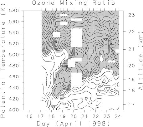
Figure 1. Time-height section of ozone mixing ratio (ppmv) over Shigaraki. The left and right axes represent the potential temperature and the approximate altitude, respectively. Regions with values larger than 1.6 ppmv are shaded. Ozonesonde observation dates are marked on the top axis.
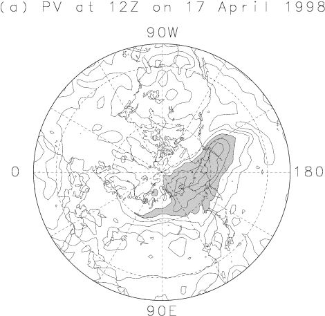
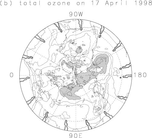
Figure 2. Polar plots of (a) potential vorticity at 460 K at 12Z on 17 April and (b) total ozone on 17 April. Contour intervals are (a) 3 PVU ( 1 PVU = 10-6 K kg-1 m2 s-1) and (b) 50 DU ( 1 DU = 2.687 × 10¹⁶ molecules of ozone per cm2). Regions with values larger than (a) 24 PVU and (b) 450 DU are shaded.
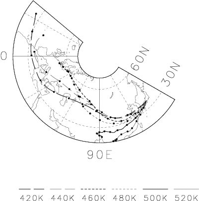
Figure 3. Backward trajectories over 10 days from Shigaraki on 6 isentropes, starting at 19Z on 19 April when the ozone mixing ratio at 460 K and 480 K was enhanced. Thick dashed, thin dashed, thick dotted, thin dotted, thick solid and thin solid lines represent the trajectories on 420 K, 440 K, 460 K, 480 K, 500 K and 520 K isentropic surfaces, respectively. Closed circles on the trajectories indicate a one-day interval.
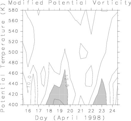
Figure 4. Same as Fig. 1 but for modified potential vorticity at 35°N, 135°E calculated with the ECMWF data. Contour intervals are 1.25 PVU. Regions with values larger than 12.5 PVU are shaded.
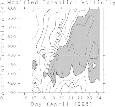
Figure 5. Same as Fig. 4 but for reconstructed MPV by RDF at Shigaraki.
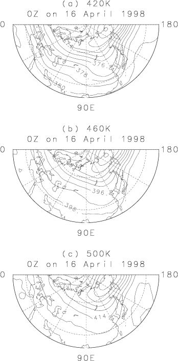
Figure 6. Montgomery potential on the (a) 420 K, (b) 460 K and (c) 500 K isentropic surfaces at 0Z on 16 April 1998 based on the ECMWF operational analysis data. Contour intervals are 103 m2 s-2.